Table Of Content

In specifying a linear mixed model, we use terms of the form (1|X) to introduce a random offset for each level of the factor X; this construct replaces the Error()-term from aov(). For our example, the model specification is then y~drug+(1|litter), which asks for a fixed effect (\(\alpha_i\)) for each level of Drug, and allows a random offset (\(b_j\)) for each litter. An appreciable block-by-treatment interaction means that the differences in enzyme levels between drugs depend on the litter. Treatment contrasts are then litter-specific and this systematic heterogeneity of treatment effects complicates the analysis and precludes a straightforward interpretation of the results.
2.7 Fixed Blocking Factors
Therefore, a block is defined by a homogenous large unit, including, raw materials, areas, places, plants, animals, humans, etc. where samples or experimental units drawn are considered identical twins, but independent. Nesting blocking factors essentially results in replication of (parts of) the design. In contrast, crossing blocking factors allows us to control several sources of variation simultaneously. The most prominent example is the latin square design, which consists of two crossed blocking factors simultaneously crossed with a treatment factor, such that each treatment level occurs once in each level of the two blocking factors.
A design of experiments Cyber–Physical System for energy modelling and optimisation in end-milling machining - ScienceDirect.com
A design of experiments Cyber–Physical System for energy modelling and optimisation in end-milling machining.
Posted: Tue, 18 Oct 2022 08:16:44 GMT [source]
ANOVA Display for the RCBD
And then, the researcher must decide how many blocks are needed to run and how many replicates that provides in order to achieve the precision or the power that you want for the test. To do a crossover design, each subject receives each treatment at one time in some order. So, one of its benefits is that you can use each subject as its own control, either as a paired experiment or as a randomized block experiment, the subject serves as a block factor. The smallest crossover design which allows you to have each treatment occurring in each period would be a single Latin square.
Identify nuisance variables
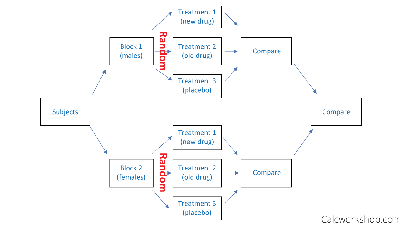
Depending on the nature of the experiment, it’s also possible to use several blocking factors at once. However, in practice only one or two are typically used since more blocking factors requires larger sample sizes to derive significant results. Gender is a common nuisance variable to use as a blocking factor in experiments since males and females tend to respond differently to a wide variety of treatments. In case all samples cannot be processed together, one first createsthe batches, and subsequently performs block randomization withineach batch. Given that we are interested in all comparisons betweenthe treatment–sex combinations, we make two batches of 12 samples,each batch containing three subjects of each group (Figure Figure55). This way, the batches arebalanced in terms of the subject-characteristics that we use in theanalytical model.
Statistical Design and Analysis of Biological Experiments
We could select the first three columns - let's see if this will work. Click the animation below to see whether using the first three columns would give us combinations of treatments where treatment pairs are not repeated. Is the period effect in the first square the same as the period effect in the second square? If it only means order and all the cows start lactating at the same time it might mean the same.
3 Incomplete Block Designs
I think that in medical context, in a two factors anova one of the factors is almost always called "treatment" and the other "block". Returning to Example 3.2, we can use these results to estimate all pairwise differences between the four treatments. Firstly, we directly calculate the \(q_j\) from treatment and block sums, using the incidence matrix. Since the first three columns contain some pairs more than once, let's try columns 1, 2, and now we need a third...how about the fourth column. If you look at all possible combinations in each row, each treatment pair occurs only one time.
The randomized complete block design can be too restrictive if the number of treatment levels is large or the available block sizes small. Fractional factorial designs offer a solution for factorial treatment structures by confounding some treatment effects with blocks (Chapter 9). For a single treatment factor, we can use incomplete block designs (IBD), where we deliberately relax the complete balance of the previous designs and use only a subset of the treatments in each block. Linear mixed models and ‘traditional’ analysis of variance use the same linear model to analyze data from a given design.
Complete Block Designs
We then replicate a full CRD in the two laboratories, leading to a design with (Lab) as a blocking factor, but multiple observations of each treatment in each laboratory. This design is helpful to account for laboratory-specific differences. As always, practical considerations should be taken into account when deciding upon blocking and randomization. There is no point in designing an overly complicated blocked experiment that becomes too difficult to implement correctly. On the other hand, there is no harm if we use a blocking factor that turns out to have no or minimal effect on the residual variance. Figure Figure11A shows the experimental setting for the ordered allocationwith Placebo subjects processed first, while Figure Figure11E shows the samesubjects in a complete randomized allocation.
What is a Randomized Block Experiment?
A microfluidic optimal experimental design platform for forward design of cell-free genetic networks - Nature.com
A microfluidic optimal experimental design platform for forward design of cell-free genetic networks.
Posted: Fri, 24 Jun 2022 07:00:00 GMT [source]
For the first six observations, we have just assigned this a value of 0 because there is no residual treatment. But for the first observation in the second row, we have labeled this with a value of one indicating that this was the treatment prior to the current treatment (treatment A). In this way the data is coded such that this column indicates the treatment given in the prior period for that cow.
Then you can randomly assign the specific operators to a row and the specific machines to a column. The treatment is one of four protocols for producing the product and our interest is in the average time needed to produce each product. If both the machine and the operator have an effect on the time to produce, then by using a Latin Square Design this variation due to machine or operators will be effectively removed from the analysis.
The inclusionof a common reference sample is especially importantwhen doing longitudinal/time-series experiments where samples areextracted from patients at multiple time-points. Processingthe samples as they become available can however introduce other confounders,e.g., machine performance or batches of chemicals. The solution isto process the samples at set time-points, and apply the same commonreference sample across the entire experiment. The common referencesample then has to be present in every batch and its placement inthe batch ought to be randomized. For a complete block design, we would have each treatment occurring one time within each block, so all entries in this matrix would be 1's.
One concrete application is a microarray study, where several conditions are to be tested, but only two dyes are available for each microarray. If all pairwise contrasts between treatment groups are of equal interest, then a BIBD is a reasonable option, while we might prefer a reference design for comparing conditions against a common control as in Figure 7.11A. By placing the individuals into blocks, the relationship between the new diet and weight loss became more clear since we were able to control for the nuisance variable of gender. Unfortunately nuisance variables often arise in experimental studies, which are variables that effect the relationship between the explanatory and response variable but are of no interest to researchers. Boxplots for the true and observed proteinabundances simulatedin Figure Figure11.
The only randomization would be choosing which of the three wafers with dosage 1 would go into furnace run 1, and similarly for the wafers with dosages 2, 3 and 4. The usual rule is to pick an effect you are least interested in, and this is usually the highest order interaction, as a means of specifying how to do blocking. In this case it is the AB effect that we will use to determine our blocks. As you can see in the table below we have used the high level of AB to denote Block 1, and the low-level of AB to denote Block 2. In addition, the block totals—calculated by adding up all response values in a block—also contain information about contrasts and effects if the block factor is random. We again refrain from discussing the technical details, but provide some intuition for the recovery of inter-block information.
For our example, we calculate three contrasts comparing each drug respectively their average to placebo. The results are given in Table 7.4, and demonstrate the differences in degrees of freedom and precision between the two underlying models. We can typically consider the levels of a blocking factor as randomly drawn from a set of potential levels.
The six treatment combinations can still be accommodated when blocking by litter, and using four litters of size six results in the experimental layout shown in Figure 7.7 with 24 mice in total. Already including a medium-fat diet would require atypical litter sizes of nine mice, however. Thus, in any experiment that uses blocking it’s also important to randomly assign individuals to treatments to control for the effects of any potential lurking variables.
Hence, with sex and treatment as the treatmentvariables, one has to make sure that the effects of both separatelyand their interaction can be estimated. For this, all combinationsof sex and treatment should be present in the experiment. Additionallythe comparison between these combinations should not be confoundedby a control variable. As a general advice, to reducethe complexity of experimental design,execution, and downstream analysis, it is recommended to keep thedistribution of control variables as simple as possible. Note thatthis also applies to sample characteristics such as sex, age, andpatient ancestry. It looks like day of the week could affect the treatments and introduce bias into the treatment effects, since not all treatments occur on Monday.


No comments:
Post a Comment